
Here’s an example where you know the exact range you want to sum, as in the following illustration.
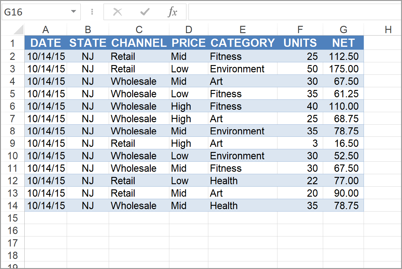
To add Sum functions for columns F and G use the following code:
Sub SumExample1()
Range(“F15”).Value = WorksheetFunction.Sum(Range(“F2:F14”))
Range(“G15”).Value = WorksheetFunction.Sum(Range(“G2:G14”))
End Sub
Notice that the WorksheetFunction.Sum method has been used.
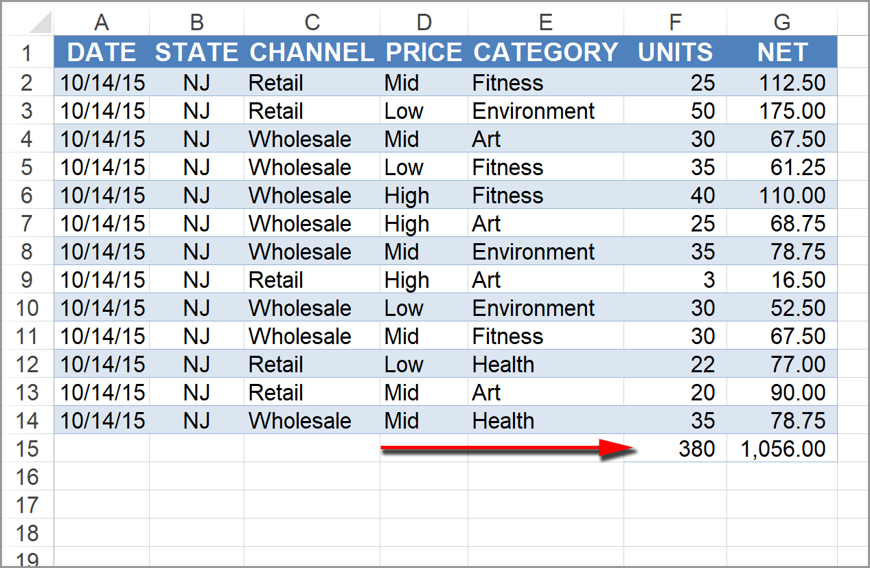
After the code runs, this will be the result:
If you don’t know the size of the range, you can use the following code:
Sub SumExample2()
Dim BottomRow As Long
BottomRow = Range(“G1048576”).End(xlUp).Row
BottomRow = BottomRow + 1
Range(“F” & BottomRow) = “Total Net”
Range(“G” & BottomRow) = Application.WorksheetFunction.Sum(Range(“G2:G” & BottomRow))
End Sub
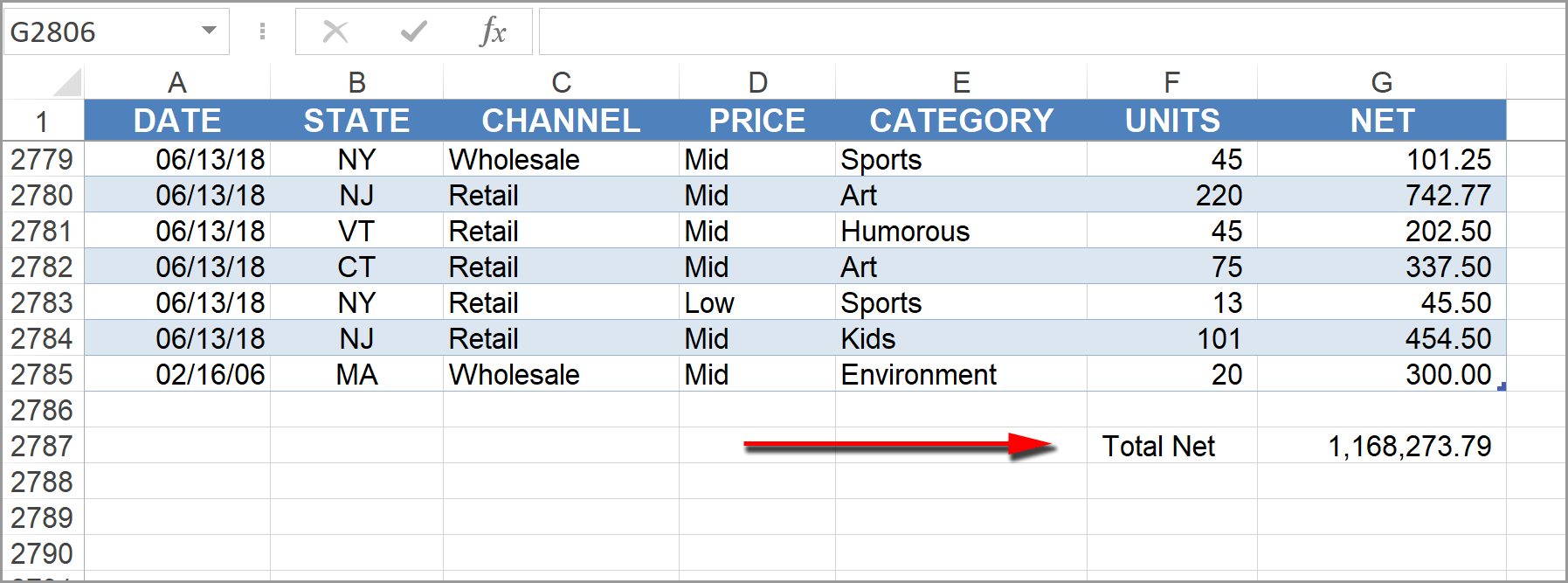
After the declaration of the variable for “BottomRow,” this code starts at the very bottom row of your spreadsheet (in my version of Excel the last row is 1,048,576). Then it jumps back up to the last filled in row and goes down two rows to skip a row between the table and the total. The ampersand (&) is the concatenation symbol to add the row number to the column letter.
In column F it will place the text, “Total Net.” In column G it will enter the sum function for all of the cells in range G2:G2785.
0 Comments